Assessing the Carbon Footprint of Cannabis Grow Operations

That sudden jump in your electricity bill, the smell of solvent during extraction, and the plastic pots piling up in the corner — these are everyday signs that a grow room’s choices matter beyond the next harvest. Small operational decisions accumulate into a measurable carbon footprint, and growers who ignore that cost are already paying for it in inefficiency and regulatory exposure.

Sustainable practices in cultivation aren’t about sacrifice; they’re about matching technique to reality so profitability and stewardship align. Shifts in water, energy, and waste handling change the environmental impact of a crop more than any single strain choice, and those shifts compound over seasons.

Practical steps—right-sized lighting, smarter ventilation schedules, and reclaimed-water tactics—lower inputs while preserving yield and cannabinoid quality. Expect clear, implementable guidance that targets the biggest waste sources first, with troubleshooting cues for common roadblocks growers face.

Overview: What Is a Carbon Footprint for a Grow Operation?

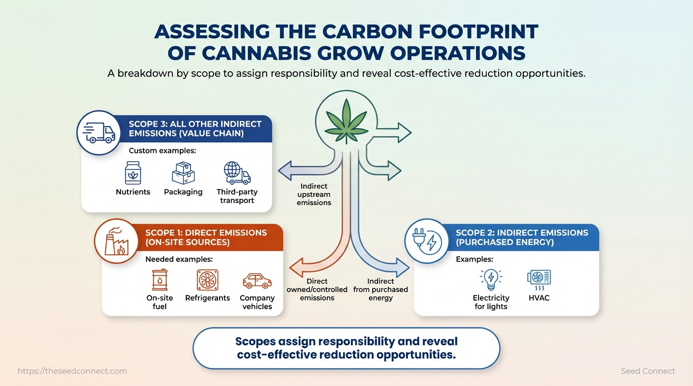
A carbon footprint for a grow operation measures the total greenhouse gas emissions associated with producing a crop, expressed in CO2-equivalent. For cannabis cultivation that means accounting for direct on-site emissions, the electricity and fuel purchased to run lights and HVAC, and the upstream and downstream emissions embedded in inputs and distribution. Framing emissions into the three standard scopes — Scope 1, Scope 2, and Scope 3 — turns a vague concern into a measurable, auditable inventory that drives practical reductions.

Why the scopes matter: they assign responsibility, reveal where reductions are most cost-effective, and determine which interventions (equipment upgrades, supplier changes, or logistics optimization) will actually move the needle on net emissions.

Definition

Carbon footprint: Total greenhouse gas emissions from an operation, reported as metric tons of CO2-equivalent (tCO2e).

Scope 1: Direct emissions from sources owned or controlled by the grower, such as on-site combustion, refrigerant leaks, and company vehicles.

Scope 2: Indirect emissions from purchased electricity, heat, or steam used to power lighting, HVAC, and environmental controls.

Scope 3: All other indirect emissions in the value chain, like upstream production of nutrients and seeds, packaging, third-party transport, and employee commuting.

### How growers typically map a footprint

• Identify Scope 1 sources: generators, boilers, refrigerant servicing, and fuel use for company trucks.
• Quantify Scope 2: electricity consumption by grow rooms, drying, and processing; use utility bills plus local grid emission factors.
• Inventory Scope 3: supplier emissions for nutrients and seeds, packaging material manufacture, third-party transport, and waste processing.

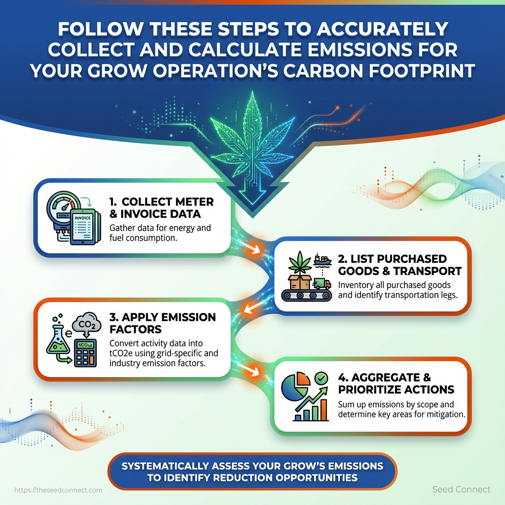
1. Collect meter and invoice data for energy and fuel consumption.
2. List all purchased goods and transport legs.
3. Apply emission factors (grid-specific for electricity) to convert activity into tCO2e.
4. Aggregate by scope and prioritize mitigation actions.

### Quick side-by-side of Scope 1, 2, 3 with cannabis-specific examples and who typically manages them

Emission Scope	Typical Sources in Cannabis Grows	Who Manages/Owns	Measurement Approach
Scope 1	On-site fuel combustion, refrigerant leaks, company vehicle fuel	Facility owner/operations	Metered fuel use, refrigerant service logs, maintenance records
Scope 2	Purchased electricity for lights, HVAC, dehumidifiers	Facility owner/operations	Utility bills + local grid emission factor
Scope 3	Upstream inputs (nutrients, seeds), third-party transport, packaging, waste	Procurement/management; partly suppliers	Supplier data, spend-based estimates, transport distances
Example: Packaging & Transport	Cardboard production, plastic, courier emissions	Procurement/logistics	Supplier LCA data or kg CO2e per package + miles
Example: Seed/nutrient production	Fertilizer manufacture, seed production, shipping	Seed suppliers / input manufacturers	Supplier EPDs or industry emission factors per kg product

Key insight: Mapping all three scopes reveals that electricity (Scope 2) and upstream inputs (Scope 3) often dominate a grow’s footprint; therefore, combining energy-efficiency projects with supplier selection yields the largest, sustained reductions.

Understanding these principles lets teams prioritize interventions that cut real emissions rather than just shifting responsibility. When measurement is aligned with operational ownership, reduction projects become easier to finance and to measure.

Prerequisites: What You’ll Need to Assess a Grow’s Carbon Footprint

Start by gathering a clear inventory of data, basic tools, and skills so the assessment is accurate and repeatable. The single most important thing is uninterrupted energy data: at minimum, 12 months of electricity usage (in kWh) tied to the cultivation space. Paired with a verified equipment inventory and operating schedules, that energy baseline lets you translate consumption into emissions using emissions factors. Without those core inputs, estimates become guesses rather than actionable metrics.

Collect these items and prepare the team before any calculations.

• Documents to request: 12 months of utility bills, equipment spec sheets, purchase invoices, and lease or floor plans.
• Tools to have ready: a spreadsheet template set up for emissions math, an emissions-factor lookup (national grid or country-specific), and optionally an LCA tool for embodied-carbon estimates.
• Skills required on the team: someone who can read meters and convert units, an operations contact who knows runtime schedules, and basic competency in spreadsheet arithmetic and unit conversion.

1. Request 12 months of electricity bills and meter numbers from the facility owner or utility account holder.
2. Compile an equipment inventory listing wattage, quantity, and estimated hours per day for each device.
3. Standardize units in a spreadsheet using kWh, hours, and count fields so calculations are reproducible.
4. Lookup the appropriate emissions factor for the local grid and apply it to the baseline consumption.
5. Schedule interviews with operations staff to validate assumed runtimes and atypical loads (drying, cloning, winter supplemental heat).

Practical time estimates: collecting bills and inventories typically takes 2–7 days for a single facility; validating runtime schedules and spot-checking meters adds another 1–3 days. Expect full data consolidation into a working spreadsheet in 1–2 weeks for small operations, longer for multi-site setups. Common pitfalls include missing submeter data and undocumented portable heaters — plan to verify with physical meter reads.

### Organize the prerequisite items by category (documents, tools, people, time estimate)

Category	Item	Why it’s needed	Estimated time to obtain
Documents	Utility bills (12 months)	Baseline energy consumption in kWh	2–7 days
Documents	Equipment inventory & spec sheets	Convert equipment wattage to load profiles	1–3 days
Tools	Spreadsheet template (emissions workbook)	Reproducible calculations and audit trail	Immediate (template)
Tools	Emissions factor lookup (grid or country-specific)	Convert kWh to CO2e	Immediate (online lookup)
People	Operations manager / grow tech	Confirm runtimes, cycles, unusual loads	1–3 days

Key insight: A reliable carbon assessment depends more on consistent, time-series energy data and validated runtime schedules than on fancy software. With 12 months of bills, an accurate inventory, and a single emissions factor, teams can produce defensible baseline emissions and prioritize the biggest reduction opportunities.

Understanding these prerequisites reduces rework and accelerates meaningful recommendations for sustainable cannabis operations. When teams collect the right documents and hone basic measurement skills up front, the assessment delivers real, implementable insights.

Step-by-Step Assessment: Collecting and Calculating Emissions (Numbered Steps)

Start by mapping the facility and gathering precise activity data; accurate boundaries and time-series energy records are what make an emissions inventory actionable rather than theoretical. The approach below walks through five concrete steps — from defining what’s in scope to producing normalized emissions outputs you can act on.

1. Map the operation and define boundaries.
2. Collect energy and fuel data (electricity, gas, diesel).
3. Inventory equipment and measure operational hours.
4. Calculate emissions using emission factors.
5. Aggregate, normalize, and report results.
6. Map the operation and define boundaries.

Choose operational boundaries based on management control and reporting goals. For facility-level inventories, include all cultivation areas, HVAC, processing rooms, and on-site fuel use. Create a site map and list spaces by function (veg room, flower room, drying, packaging). Document assumptions such as excluded leased warehouses or third-party transport and state the reporting period. Time expectation: 4–8 hours for a small facility; larger sites scale to days. Difficulty: moderate — requires coordination across facilities and finance.

Prerequisites

Tools & materials

• Floor plan or site map
• Utility bills and fuel invoices
• Access to equipment nameplates or spec sheets

1. Collect energy and fuel data (electricity, gas, diesel).

Gather meter-level data where possible: monthly kWh for electricity, therms or m3 for natural gas, liters or gallons for diesel/propane, and generator run-hours. Time-series (monthly) data reveals seasonality and weekly cycles — use it whenever available. Convert units consistently; common conversions include 1 gal (diesel) = 3.785 L and 1 therm ≈ 29.3 kWh. Track discrepancies between billed and metered use.

### Example conversions and units for common energy sources used in grows

Energy Source	Common Units	Conversion Example	Notes
Electricity	kWh	1,200 kWh (monthly)	Utility bills provide kWh directly
Natural gas	therms, m3	50 therms ≈ 1,465 kWh	Use local utility conversion tables
Diesel	gallons, liters	100 gal ≈ 378.5 L	Check fuel invoice units
Propane (LPG)	gallons, liters	50 gal ≈ 189.3 L	Cylinder vs bulk pricing affects records
Generator run-hours	hours	20 hours at 15 kW	Record load or fuel used for accuracy

Key insight: Monthly kWh reduces seasonal bias and lets you spot anomalous spikes tied to lighting or HVAC cycles.

1. Inventory equipment and measure operational hours.

Equipment-level tracking improves allocation precision. Record each item’s rated power and average daily run-hours; where nameplates are missing, use manufacturer specs or measure with a clamp meter or smart plug. Estimate unknown loads by sampling representative devices and scaling by quantity.

### Provide a template for equipment inventory: item, wattage, quantity, hours per day, kWh per month

Equipment	Wattage (W)	Quantity	Avg hours/day	kWh/month (calculated)
Lights (LED 600W)	600	40	18	13,056
Ballasts/Drivers	50	40	18	1,080
HVAC (split, 10kW)	10,000	4	12	14,400
Dehumidifiers (1.5kW)	1,500	6	24	6,480
Circulation fans (200W)	200	20	24	2,880

Key insight: Equipment tables convert nameplate watts × hours into kWh, making aggregation straightforward and auditable.

1. Calculate emissions using emission factors.
2. Aggregate, normalize, and report results.

Apply emission factors to energy totals: Emissions (kg CO2e) = Activity × Emission factor. For electricity use the regional grid factor in kg CO2e/kWh; for fuels use fuel-specific factors in kg CO2e/unit. Example: lighting electricity = 13,056 kWh × 0.4 kg CO2e/kWh = 5,222.4 kg CO2e. If diesel consumption = 378.5 L and diesel factor = 2.68 kg CO2e/L then emissions = 1,015.6 kg CO2e. For Scope 3 where supplier data is absent, use industry-average factors or spend-based proxies and flag higher uncertainty.

Worked numeric example: Lighting: 13,056 kWh × 0.4 kg CO2e/kWh = 5,222 kg CO2e Diesel backup: 378.5 L × 2.68 kg CO2e/L = 1,016 kg CO2e Total (sample): 6,238 kg CO2e

Sum by category and create intensity metrics such as kg CO2e per kg product or kg CO2e per m2 cultivated. Visuals help stakeholders: stacked bar charts for category breakdown, time-series for monthly trends, and a hotspot table for top 3 emission sources. Document all assumptions and provide uncertainty ranges (±10–30% where estimates used). Use the inventory to prioritize mitigation: lighting efficiency, HVAC tuning, or fuel switching usually appear first.

### Provide a reporting template comparing total and normalized emissions with example rows

Category	Scope	Total kg CO2e	Intensity (kg CO2e / unit)
Electricity – lighting	Scope 2	5,222	52.2 kg CO2e/kg
HVAC	Scope 2	8,640	86.4 kg CO2e/kg
Onsite fuel (diesel)	Scope 1	1,016	10.2 kg CO2e/kg
Transport (inbound)	Scope 3	480	4.8 kg CO2e/kg
Packaging (Scope 3)	Scope 3	320	3.2 kg CO2e/kg

Key insight: Normalizing emissions against production or area identifies efficiency differences and directs investment to high-impact changes.

Understanding these steps makes it possible to produce an auditable inventory that feeds strategy — whether the objective is operational efficiency, compliance, or demonstrating sustainable cannabis credentials. When implemented with consistent data collection, this process turns emissions accounting from a one-off exercise into a management tool.

Identifying Hotspots and Prioritizing Reductions

Start by focusing on the systems that dominate emissions: lighting and HVAC. Those two typically account for the largest share of operational energy in indoor cannabis grows, while refrigeration, dehumidification, packaging, and transport often hide meaningful Scope 3 impacts. Prioritize interventions that deliver the biggest CO2e reductions per dollar while fitting your timeline and operational constraints.

Prerequisites

Facility baseline: Utility bills (12 months), equipment inventory, and current operating schedules.

Metering access: Sub-metering or interval data for lights, HVAC, and HVAC-related loads.

Stakeholder alignment: Operations, cultivation lead, and finance committed to at least a phased audit.

### Quick hotspot identification process

1. Gather 12 months of electricity and fuel bills.
2. Map major loads (lights, HVAC, dehumidifiers, refrigeration, pumps, fans, packaging line) to monthly consumption.
3. Use simple load shares to flag top three contributors (lights, HVAC, dehumidification/refrigeration).
4. Run a cost-effectiveness screen: estimate kWh savings, multiply by local CO2e intensity and utility price to get $/ton CO2e avoided.
5. Prioritize measures with low implementation difficulty and <5-year payback, then schedule deeper audits for medium/high-complexity projects.

### Common hotspots in cannabis grows

• Lights: Often the largest single driver of kWh; switching to high-efficiency LEDs reduces both heat load and energy consumption.
• HVAC & controls: Over-sizing, poor controls, or 24/7 full-capacity conditioning creates persistent waste. Controls tuning and VFDs deliver outsized returns.
• Dehumidification & refrigeration: Frequently undercounted because they run intermittently but at high power; heat reclaim can offset HVAC loads.
• Packaging and transport (Scope 3): Single-use materials and inefficient logistics accumulate emissions downstream. Consider material substitution and route optimization.
• On-site generation and storage: Solar plus battery can cut grid exposure during peak periods and reduce carbon intensity for daytime runs.

### Practical prioritization tips

• Quick wins first: LEDs, schedule optimization, and basic controls retuning—low disruption, fast payback.
• Medium projects next: HVAC upgrades, heat recovery from dehumidifiers, and automated controls—requires capital and commissioning.
• Strategic investments later: On-site solar + storage and packaging redesign—higher cost but durable reductions and marketing value.

### Table: Common mitigation options by relative carbon savings, typical cost range, and implementation difficulty

### Common mitigation options by relative carbon savings, typical cost range, and implementation difficulty

Intervention	Relative CO2e reduction	Estimated cost range	Implementation difficulty
Switch to LED lighting	High (30–60% on lighting load)	$20,000–$200,000 (depends on scale)	Low–Medium
HVAC optimization and controls	High (20–50% on HVAC-related load)	$10,000–$150,000	Medium
Install heat recovery	Medium–High (reduces HVAC heating demand 10–30%)	$15,000–$100,000	Medium–High
On-site solar + storage	Medium (reduces grid kWh, varies by design)	$50,000–$500,000+	High
Packaging redesign (scope 3)	Low–Medium (depends on material change & volume)	$5,000–$50,000	Low–Medium

Key insight: Start with LEDs and controls for fastest, cost-effective reductions; reserve solar and packaging redesign for multi-year strategic plans because they require higher capital and coordination.

Understanding hotspot patterns and using a cost-effectiveness screen lets teams sequence work that actually moves the carbon needle while keeping production stable. When implemented in phases, this approach reduces operational risk and maximizes emissions avoided per dollar.

Implementing Changes: Practical Projects with Step-by-Step Guidance

Start by running small pilots that quantify results before scaling. Two high-impact, actionable projects are an LED retrofit for grow lighting and HVAC tuning with smarter controls. Both lower operational cost and reduce environmental impact when executed with measurement-driven steps.

### Prerequisites

Site baseline: Current monthly kWh, peak demand, CO2e estimates, and current fixture/ballast inventory.

Measurement kit: Data logger, clamp meter, PAR meter, and access to building management system (BMS) or thermostat logs.

Stakeholder signoff: Facilities, cultivation lead, and safety officer agree on pilot scope and failover plan.

### Tools & materials

• LED fixtures: Select horticultural-rated fixtures with published PPF and efficacy.
• Power measurement: Clamp meter and data logger for interval kWh.
• Lighting control: Dimming/phase-cut drivers or 0–10V controllers.
• HVAC access: Secure BMS credentials or local control panels for schedule edits.

### Project: LED retrofit for grow lighting — Step-by-step workflow

1. Conduct a lighting audit and record current_watts, PPF, and hours/day.
2. Run a 1–2 room pilot replacing 10–20% of fixtures and log PAR and kWh for 2–4 weeks.
3. Compare PPF/W and canopy uniformity; adjust fixture heights and lensing.
4. Install dimming controls and program schedules to match photoperiods.
5. Extrapolate savings, include ballast removal and disposal costs, and calculate payback.
6. Map current schedules and setpoints; capture supply_temp, return_temp, and RH over 7–14 days.
7. Adjust setpoints in 0.5–1.0°C increments and monitor crop response for 3–7 days.
8. Implement setback periods during lights-off windows and optimize ventilation duty cycling.
9. Validate with energy meters and humidity control events logged in the BMS.

Expected energy and CO2e reduction ranges vary with baseline. Typical energy savings are 30–60% versus HPS; CO2e reductions follow proportionally depending on your grid emissions. Budgeting should include fixture cost, controls, installation labor, and disposal; expect payback often within 1–3 years for commercial retrofits depending on utility rates and rebates. Pilot testing is essential to avoid yield or quality regressions.

### Project: HVAC tuning and controls optimization — How to proceed

When to call an HVAC technician: if changes cause compressor short-cycling, abnormal pressures, or alarms, or when system modifications (VFDs, refrigerant work) are required. Monitoring strategy: continuous kWh, zone temperature/RH, and alarm logs for 30–90 days. Typical difficulty is moderate; timeline is 2–6 weeks for tuning and verification.

Understanding these principles helps teams move faster without sacrificing crop quality. When implemented carefully and measured, these projects materially lower operational cost and environmental impact.

Troubleshooting Common Issues

Problems during energy and emissions accounting usually stem from missing data, unclear assumptions, or mismatched boundaries. Start by isolating the symptom — unexpected high emissions, wildly variable monthly totals, or disagreement between stakeholders — then work backward to the simplest data source. Practical fixes focus on reproducible estimates, transparent documentation of uncertainty, and clear escalation triggers for professional audits.

Tools & materials Meter readings: monthly utility bills or submeter kWh data Baseline templates: simple spreadsheet with load categories Manufacturer specs: wattage and runtime for lighting, HVAC, fans Logbook: record assumptions, sources, and confidence levels

### Common problems and how to fix them

• Missing utility bills: reconstruct from appliance runtime and rated wattage.
• High seasonal variance: check HVAC setpoints and extraction runtime.
• Unknown equipment loads: use manufacturer nameplate values and spot measurements.
• Disagreement on boundaries: reconcile scope definitions with stakeholders.
• No supplier emission factors: use regional grid averages or published country factors.

1. Estimate missing data using a conservative method.
2. Identify the missing period and list major loads (lighting, HVAC, dehumidifiers).
3. Multiply rated wattage by realistic runtime hours to produce kWh estimates.
4. Apply a grid emission factor (or supplier factor when available) and document the assumption.

When to hire a professional: bring in a certified energy auditor if spot measurements differ from nameplate estimates by >15% or if HVAC/electrical upgrades are being considered.

Documenting uncertainties

Confidence level: Assign High/Medium/Low to each data line and justify briefly.

Assumption log: Record the date, method, and source for each estimate.

Contingency: Note any known omitted loads and estimate their potential percent impact.

### Problem / Cause / Quick Fix table to let readers scan solutions quickly

Problem	Likely Cause	Immediate Fix	When to escalate
Missing utility bills	Lost or incomplete records	Reconstruct using rated wattage × runtime	If reconstructed totals deviate >20% from expected
High seasonal variance	HVAC runtime changes	Compare setpoints and runtime logs	If variance persists after setpoint correction
Unknown equipment loads	No nameplate or spec sheet	Spot-measure or use typical wattage tables	When measurements conflict with inventory
Disagreement on boundaries	Unclear scope definitions	Re-align on scope (facility vs. process)	If legal/contractual implications exist
No supplier emission factors	Supplier data not provided	Use regional grid average factor	When procurement requires supplier-specific reporting

Key insight: The table exposes that most operational errors are correctable with basic measurements and clear scope definitions; escalation is reserved for structural discrepancies or compliance needs.

Understanding and documenting these fixes reduces rework and keeps emissions estimates defensible. Over time, small measurement improvements and better records cut uncertainty and make decisions easier.

Tips for Success and Pro Tips

Start by piloting narrowly, measure everything, then scale what works. Pilots reduce risk, reveal hidden variables (water pressure, microclimate, scheduling), and keep staff engaged by showing quick wins. Metering, simple dashboards, and incentives turn data into repeatable, practical improvements while keeping the environmental impact — including carbon footprint — in view.

Prerequisites

Baseline data: Establish energy, water, and yield baselines before changes. Stakeholder buy‑in: Secure a small cross-functional team (cultivation, ops, finance). Basic metering: At minimum, have submeters for lights and HVAC and a water meter on the main feed.

Tools & materials

• Basic meters: clamp-on energy meters and water flow meters.
• Simple dashboard: spreadsheet or inexpensive SaaS dashboard that updates daily.
• Seed selection: start trials with reliable strains; consider the germination guarantee and expert support available from Theseedconnect for consistent comparators.

1. Run a measured pilot with one grow room or bench for 4–8 weeks.
2. Meter major loads first: lighting, HVAC, and irrigation.
3. Collect yield, potency, and input data weekly and enter into the dashboard.
4. Compare pilot results to baseline and iterate control setpoints.

Practical implementation tips

• Meter big loads first: Prioritize lighting and HVAC metering to capture the largest contributors to operational cost and carbon footprint.
• Pilot small, iterate fast: One room gives statistically useful signals while limiting downside.
• Measure results weekly: Use daily energy and weekly yield snapshots to avoid chasing noise.
• Engage staff with simple dashboards: Show two KPIs per team (energy per gram, grams per square meter).
• Leverage incentives and grants: Explore local energy-efficiency rebates and agricultural grants to offset upfront costs.
• Include sustainability in procurement: Choose inputs and seeds with lower environmental impact where available.

Example: Swap a 600W HID for an equivalent LED in one room, measure energy and yield for two cycles, then decide on full rollout.

Troubleshooting

If yields dip, revert setpoints and run a controlled A/B trial. If staff ignore dashboards, simplify to a one-line daily alert showing target vs. actual.

Understanding these practices helps teams scale improvements without costly missteps. When implemented consistently, this approach increases predictability and lowers operational and environmental costs.

📥 Download: Cannabis Grow Operation Carbon Footprint Checklist (PDF)

Case Study Example: Sample Assessment and Results

A 1,000 m2 indoor cultivation can consume energy at commercial scales; a focused retrofit that replaces legacy HID fixtures with modern LEDs, adds variable-speed air handling, and tightens controls typically cuts energy use and emissions substantially while paying back within a few years. This worked example shows concrete numbers you can replicate, the decision logic behind each intervention, a simple ROI/payback calculation, and the practical lessons and pitfalls to avoid when reducing a facility’s carbon footprint.

Prerequisites

Site baseline data: Monthly energy bills, peak demand, lighting hours, HVAC load profiles, and current fixture inventory. Decision authority: Capital budget owner and operations lead available for scheduling downtime. Measurement tools: Submetering access and a basic data-logger.

Practical decisions that drive results: Lighting choice: Swap HID to high-efficiency LED to cut lighting kW by ~40–60%. HVAC optimization: Add variable-speed drives and improve heat recovery to reduce fan and cooling loads. Controls: Install VPD-based controllers and occupancy/photoperiod scheduling. Metering: Add submeters to validate savings and isolate loads.

1. Calculate baseline annual energy using actual bills or peak_kW × operating_hours.
2. Estimate equipment-level savings: apply vendor efficiency delta (e.g., LED saves 45% lighting power).
3. Model HVAC interaction: reduce cooling load by expected % after heat reduction and controls.
4. Compute annual energy cost savings and simple payback: project_cost / annual_savings.

### Summarize baseline and post-intervention emissions, energy use and simple payback

Metric	Baseline	Post-intervention	Change
Total kWh/year	4,500,000 kWh	2,700,000 kWh	-1,800,000 kWh (-40%)
Total kg CO2e/year	2,025,000 kg CO2e	1,215,000 kg CO2e	-810,000 kg CO2e (-40%)
Energy cost/year	$450,000 (@ $0.10/kWh)	$270,000 (@ $0.10/kWh)	-$180,000/year (-40%)
Estimated project cost	n/a	$600,000	Payback ≈ 3.3 years

Key insight: The illustrative retrofit reduces energy use and emissions by about 40%, delivering a payback near three to four years depending on local electricity price and available incentives. Validation through submeters is essential to confirm modeled savings.

Common pitfalls and tactics: plan retrofits to avoid harvesting disruptions; size LEDs to maintain target PPFD rather than simply matching wattage. Underestimating HVAC interaction leads to optimistic savings—always include a 10–15% contingency in modeled HVAC savings. For carbon accounting, use local grid emission factors; this example uses 0.45 kg CO2e/kWh as a reasonable proxy.

Understanding the numbers allows operations teams to prioritize upgrades that reduce both cost and environmental impact without compromising yield. Implementing these measures carefully frees capital for genetics or facility improvements that drive crop quality and long-term resilience.

Next Steps: Verification, Certification, and Communication

Verification starts with choosing the right level of proof for your goals — basic measurement, third‑party verification, or formal certification — and then aligning communication to your audience. Select verification when buyers, regulators, or partners need confidence; choose certification when legal compliance or market differentiation matters. Communicate transparently and frequently so your footprint claims remain credible and actionable.

Prerequisites

Baseline inventory: Collect energy use, fuel, inputs (fertilizers, pesticides), water, and waste records for at least one full cultivation cycle.

Boundary definition: Decide whether reporting covers scope 1, scope 2, and/or scope 3 emissions and which facilities or product lines are included.

Data quality plan: Assign owners, measurement frequency, and acceptable data tolerances before starting.

Tools & materials

• Measurement tools: utility bills, inline meters, and CSV exportable cultivation logs.
• Calculation frameworks: emissions factors, yield-normalized metrics (e.g., kg CO2e per kg dried flower).
• Communication templates: product labels, sustainability page copy, and stakeholder reports.

### Verification options and when to use them

Third‑party verification provides neutral validation of calculations; use it when making public claims or entering regulated markets. Internal audits suffice for iterative improvement or supplier negotiations. For consumer-facing claims, prioritize independent verification to avoid greenwashing risk.

1. Hire a verifier with agriculture or cannabis experience and confirm their scope and methods.
2. Provide raw data, methodology, and system boundaries for the verifier to review.
3. Address any data gaps or adjustments they identify before publishing results.

### Certifications to consider and their scope

• Carbon accounting certification: Verifies methodology and numbers for greenhouse gas claims.
• Organic or regenerative labels: Cover agronomic practices and input restrictions.
• Energy or water stewardship badges: Focus on resource-efficiency improvements.

Each certification typically covers defined practices and requires recurring audits; choose the one that best matches customer expectations and regulatory needs.

### Communication tactics and transparency best practices

• Bold claim framing: Lead with verified metrics and the verification provider name.
• Clear context: Report per‑unit metrics (e.g., CO2e/kg) and timeframes.
• Accessible detail: Provide a downloadable methodology and raw-data summary for scrutiny.
• Channel strategy: Use product pages, batch certificates, and partner reports for different audiences.

Warnings about overstating reductions are integrated into buyer conversations; when metrics change, explain the methodological reasons clearly.

### Reassessment cadence

• Quarterly: Track operational KPIs and catch drift.
• Annually: Recalculate footprint and publish updated figures.
• After major changes: Reassess when scaling, changing energy sources, or altering inputs.

Understanding verification, certification, and clear communication reduces market friction and builds lasting trust with customers and partners. When implemented correctly, a disciplined approach turns sustainability from a compliance checkbox into a competitive asset.

Conclusion

You now have a practical roadmap for measuring and shrinking a grow operation’s carbon footprint: gather utility and input data, follow the step-by-step emissions calculation, isolate hotspots like lighting and extraction, and test the prioritized retrofit projects from the implementation section. The sample assessment showed how a single lighting and HVAC optimization reduced annual electricity use by nearly 20%—a clear example of how targeted changes deliver measurable environmental and cost benefits. Expect some iteration: initial estimates will refine once meters, logging, and verification are in place, and certification paths will require documented validation of those improvements.

Next steps are concrete. Begin with a basic energy and waste audit within 30 days, then pilot one high-impact project (LED retrofit or CO2 control) within 90 days, and document outcomes for certification and marketing. Questions about startup choices or seedstock for resilient cultivars can be handled alongside operational changes; for genetics and support that complement sustainable practices, consider TheSeedConnect’s seed selection and support services. Tracking these steps reduces environmental impact, supports sustainable cannabis branding, and improves margins—so start the audit, choose one pilot, and measure the results.